|
URL original: |
Conteúdo:
What is Maple V?......................................................................................................................... 2
About These Pages....................................................................................................................... 3
Maple: The Basics......................................................................................................................... 3
Numerical Calculations.................................................................................................................. 4
Graphics:....................................................................................................................................... 6
Algebraic Calculations................................................................................................................. 12
Calculus...................................................................................................................................... 15
Differential Equations................................................................................................................... 17
Matrix Operations and Linear Algebra......................................................................................... 18
Special Mathematical Functions................................................................................................... 20
Statistics...................................................................................................................................... 25
Programming............................................................................................................................... 26
Other Maple Resources............................................................................................................... 29
|
|
The Cluster Team Presents A Maple Tutorial |

![]()
![]() What is Maple?
What is Maple?
![]() About these pages
About these pages
![]() Maple: The basics
Maple: The basics
![]() Numerical Calculations
Numerical Calculations
![]() Graphics: 2-D and 3-D plots
Graphics: 2-D and 3-D plots
![]() Algebraic Calculations
Algebraic Calculations
![]() Calculus
Calculus
![]() Differential Equations
Differential Equations
![]() Matrix Operations and Linear Algebra
Matrix Operations and Linear Algebra
![]() Special Mathematical Functions
Special Mathematical Functions
![]() Statistics
Statistics
![]() Programming
Programming
![]() Maple on the Web and Books on Maple
Maple on the Web and Books on Maple
![]()
![]()
![]() Tutorials on Maple,
Mathematica, and Load Sharing Facility (LSF).
Tutorials on Maple,
Mathematica, and Load Sharing Facility (LSF).
![]() This page Maintained by Dale H. Leschnitzer (Last Modified
This page Maintained by Dale H. Leschnitzer (Last Modified
L O S A L A M O S N A T I O N A L
L A B O R A T O R Y
Operated by the
Copyright © 1999 UC - Disclaimer
![]()
![]()
Maple V is a powerful mathematical problem-solving and visualization system used world-wide in education, research, and industry. Its principal strength is its symbolic problem solving algorithms. Unlike conventional math software, which can only work with floating-point numbers, Maple V can solve problems involving formal mathematical definitions and return answers as mathematical objects. Derived from over a decade of world-class R&D and customer service, Maple V Release 4 provides all the right tools for users in education, research, and industry.
Maple is a product of the Waterloo Maple Software Corporation. Currently, the Open Cluster is running release 3.
Maple supports a plethora of mathematical systems and procedures including:
![]() Numerical Calculations
Numerical Calculations
![]() Calculus
Calculus
![]() Equation Solving
Equation Solving
![]() Trigonometric and Exponential/Logarithm
Functions
Trigonometric and Exponential/Logarithm
Functions
![]() Linear Algebra
Linear Algebra
![]() Statistics
Statistics
![]() 2d and 3d Plotting
2d and 3d Plotting
![]() Animation
Animation
![]() Interface with C and Fortran Programming
Interface with C and Fortran Programming
Maple is fairly easy to get started in. It can rapidly become a freehanded mathematical sketch pad for the user.
NOTE: Maple and the Maple Logos are trademarks ® and copyrighted © to the Waterloo Maple Software Corporation. I believe in giving credit where credit is due. Many of the examples found in these pages are based loosely upon examples from the downloadable (yet noninteractive) Maple demo or from the Maple V books published by Springer-Verlag. These two resources were helpful to me to get started in Maple and I am appreciative. These pages are for official use for Los Alamos National Laboratory Employees and authorized users of Los Alamos National Laboratory Network Compute Servers. They may not be copied without prior consent from the author.
![]()
The Cluster Team wanted to be sure its users have ample opportunity to use Maple. It was decided that a short demonstration of the application be given to show users the power behind this product.
This is by no means a complete demonstration of Maple's powerful capabilities. Instead, this demonstration is meant to whet your appetite into the fast growing world of Maple.
At the end of this lesson is a listing of Maple Web sites and books. Please browse this section.
This tutorial was written for you, the user. We would like to hear your comments. Please e-mail us at cluster-consult@lanl.gov with any suggestions for improving this tutorial. Likewise, please let us know if you would like to see other tutorials like this for other available Cluster Applications (Mathematica, NCAR, etc).
These pages have many graphics obtained from actual screens of Maple. If you do not run Maple as an X-Window application (as covered in the next lesson) your views may differ slightly.
![]()
Maple can run in either an ASCII terminal mode or as an X-window System client. To run Maple from an ASCII terminal, type maple. To run Maple as an X-window System client, type xmaple or maple -x. For help on using X-window clients, please see "Connecting to X-window System Clients." Most of the examples shown in this tutorial are taken from the X-windows session. The paths to the executables are:
(Maple ASCII executable)
/usr/bin/maple
(Maple X-windows executable)
/usr/bin/xmaple
Maple has an internal help capability that can be accessed by issuing ? at the Maple prompt and then the topic for which you want help. For example, typing ?int opens a window containing the help page for the Maple routine int. Another way to bring up a help page is to use the help browser. The browser is accessed through the Help menu in the top right corner of the Maple window. You can run the Maple tutorial by starting up maple and entering the Maple command: tutorial(); Executing man maple displays the man page for Maple.
The actual Maple session is conducted on a page called the worksheet. The worksheet can be a rather informal sketch pad or a formalized document ready for use as a figure in a publication. Maple worksheets use the greater than prompt (>). Do not try to type this prompt when duplicating the examples given in this tutorial. All commands are terminated with a semicolon (;). Plots and animations are displayed in separate windows. The worksheets and graphical output can all be saved as separate files in a variety of formats including PS, LaTeX, and GIF.
Some of the graphics displayed in this tutorial are presented as "thumbnail" sketches. This is because they are too large to display in great detail on the screen. Clicking on these images (they will be outlined as a link) will produce the larger, more detailed image.
![]()
![]()
Maple performs mathematical calculations swiftly and accurately. Unlike a calculator, Maple's worksheet can keep a permanent record of your calculations for later use.
> 123.4*8.2^3;
68038.8112
> (23.4*43)/(43.5-(3.2*2))+(12.4*34.8);
458.6412938
Maple also recognizes many special operators such as factorial, square roots, least common divisor, etc. For example:
> 13!;
6227020800
> (5^8)/(3*Pi^2)*sqrt(5);
1/2
5
390625/3 ----
2
Pi
Note that Maple kept answer in the form of an expression, i.e., it does not round off the answer. Maple will allow this expression to carry over as is so that rounding errors do not plague the user. If one wants to see the final answer as a decimal floating point, the evalf command can be used. Also note that the quotation mark (") is used to represent the last expression computed:
> evalf(");
29500.13725
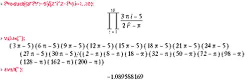
Maple also calculates finite and infinite sums and products:
> Sum((2*i+5)/(3*i^2-5),i=1..10);
10
-----
\
2 i + 5
) --------
/ 2
----- 3 i - 5
i = 1
> value(");
29392799449
- -----------
48571966058
> evalf(");
-.6051391746
> Product((3*Pi*i-5)/(2*i^2-Pi),i=1..10);
10
--------'
' |
| 3 Pi i - 5
| |
----------
| |
2
| | 2
i - Pi
i = 1
> value(");
(3 Pi -
5) (6 Pi - 5) (9 Pi - 5) (12 Pi - 5) (15 Pi - 5) (18 Pi - 5)
/
(21
Pi - 5) (24 Pi - 5) (27 Pi - 5) (30 Pi - 5)
/ ((2 - Pi) (8 - Pi)
/
(18
- Pi) (32 - Pi) (50 - Pi) (72 - Pi) (98 - Pi) (128 - Pi) (162 - Pi) (200 - Pi))
> evalf(");
-1.089588169
Notice the above gets a little messy on an ASCII screen. Lets take a look at it as it appears on an X-Window session:
One can round off the value to any number of decimal places desired:
> 5/3;
5/3
> evalf(",3);
1.67
Maple also utilizes complex numbers:
> (12+8*I)*(9+3*I)/(2+I);
276/5 + 132/5I
![]()
![]()
![]() 2-D Plots
2-D Plots
![]() 3-D Plots
3-D Plots
![]() Saving and Printing
Plots
Saving and Printing
Plots
One can develop a multitude of plots with Maple. These plots can be function based, point-by-point based, or any combination of the two. One has a great deal of power in the plot formats. For example, one can specify discontinuous plots (i.e., a plot of the tan function), hide and shade surfaces, normalize axis, etc.
Here is a simple parabola:
> plot((3*x^2-4),x=-10..10);
A 300 + A
AA + AA
AA + AA
AA 250
+ A
A
+ A
A
+ A
AA
+ AA
A 200 + A
A + A
A + AA
AA 150 + AA
AA + AA
AA + AA
AA + AA
AA 100 + AA
AAA + AAA
AAA + AAA
AA 50 + AAA
AAA + AAA
AAA
+ AAA
AAAAA +
AAAAA
+---+--+---+---+--+---+---+---+-***********-+---+---+---+---+---+---+--+---+
-10 -5 0 0 5 10
On an X-Window session, Maple opens up a second window containing the plot:
To plot two or more functions on one graph, enclose the functions in curly brackets {}. One can define both the x and y values:
> plot({sin(x),x-x^3/6+x^5/120},x=-4..4);
+ A
+ A
1.5 + + AA
+ A
1 + ********** A
B
+ *** B*** AA
BB + *** B**AAA AAA
BB 0.5 + ** BB AA
BB + ** BB
BB +* BB
+---+--+**-+---+--+---+---+---+--+-***---+--+---+---+---+--+---+--**--+---+
-4
BB -2 *0 0 2 BB
4
AAA BB -0.5 + BB
AAA
AAA*BB *** + BBB
AA
A***B ***
+
B
A ********** -1 +
AA
+
AA
+
A -1.5 +
A +
A +
Discontinuous and step functions can also be easily displayed:
>
plot(tan(x),x=-2*Pi..2*Pi,-4..4,discont=true);
C C 4 +
C C
CC C +
C C
C C +
C C
C C +
C C
C C +
C C
CC C
2 + CC C
C CC +
C CC
CC CC +
CC C
CC CC +
CC CC
CCC CC + CCC CC
***-+-+--+-+-+--+-+**--+-+--+-+-+--+-***--+-+-+--+-+--+-**+--+-+-+--+-+-+--
CC CC* CC CCC
-6 -4 CC -2
CC0 0 2 CC 4
CC6
CC CC +
CC CC
C CC +
CC CC
CC C +
CC C
C CC
-2 + C CC
C C +
C C
C C +
C C
C C +
C C
C C +
C C
C C -4 +
C C
Maple allows one to compute much more complex plots such as polar, spherical, and cylindrical coordinates, conformal plots for complex functions, and other specialized graphics. To load these features, use the with(plots) command.
Lets look at a polar plot:
> with(plots, polarplot);
[polarplot]
> plots[polarplot](t);
AAAAAAAAA 1.8 + AAAAAAAAA
AAA AAA
+ AAA AAAA
AAA AAA+AAA AAA
AA 1.6A*A A
AAA A+A AAA
AA 1.4 + AA AA
A AA +
AA A
AA 1.2 + A AA
A A
+ A A
A AA 1 +
AA A
A A +
A A
AA A +
A AA
AA A 0.8
+ A AA
A A +
A A
AA A 0.6
+ A AA
A A +
A A
AA A 0.4
+ A AA
A
AA + AA A
AA
A + A AA
A A0.2 + AA A
A AA +
A A
-*-+-+--+-+-+-+--+-+-+-+--+-+-+-+--*****--+-+-+-+--+-+-+-+--+-+-+-+--+-+-*-
-3 -2 -1 0
0 1 2 3
![]()
Note: All 3-D plots will be shown as X-Window Session Images.
One can plot surfaces and 3-dimensional objects with Map0pt;mso-bidi-font-family:"Times New Roman"'>plot3d command. You need to define all of the variables in your plot3d statement. For example:
>plot3d((x^3)*sin(a*x^2),a=0..5,x=0..3,axes=BOXED);
Once the window opens with the plot, the mouse may be used to rotate the graph into any orientation. Pull-down menus allows one to choose between different surface renderings (hidden line, patch, contour, etc) and different light/color schemes. Some of these features are shown in the next figures.
A nice feature of Maple is the ability to graph an equation without having to first solve the equation based on any one variable. The implicitplot3d command is the way to invoke this feature:
>with(plots);
>implicitplot3d(x^3+5*y^2-z^3-8=0,x=-10..10,y=-10..10,z=-10..10);
The resulting surface is displayed below. Note that we can alter how the plots looks very easily:
One also has the option of plotting curves and surfaces defined parametrically. Let us define (for more information on functions, see Lesson 6, Algebraic Calculations) three functions, F,G, and H:
>F:=(u,v) ->
sin(u)*cos(v);
>G:=(u,v) ->
sin(u)*sin(v);
>H:=(u,v) -> cos(u);
Now letÕs plot these three functions parametrically as a solid surface. We shall constrain the scaling to preserve our true spherical shape. Note that we will include the three functions in square brackets []:
plot3d([F,G,H],0..Pi,0..2*Pi,style=PATCH,scaling=CONSTRAINED);
(we could have performed the entire feat in one statement):
>plot3d([sin(u)*cos(v),
sin(u)*sin(v),cos(u)],u=0..Pi,v=0..2*Pi,style=PATCH,scaling=CONSTRAINED);
Error! Filename not specified.Expand
![]()
As you have probably seen by now, the prefered method for displaying graphics is through an X-window session. But this does not mean that one cannot generate great looking plots via a text-only session. It just takes a little planning.
First off, you need to define your output style. Usually, this will be a postscript® file. Next, you will need to define the output file name. The interface command is used to set both of these paramaters:
>interface(plotdevice=postscript,plotoutput=myfile.ps);
Now, when you plot the graph, the output will go directly to the file. If you are ready to plot a second graph, be sure to specify a new file name:
>interface(plotoutput=myfile2.ps);
If you use the X-Windows Maple interface there is a pulldown menu that you can take advantage of. Under File there is a second menu called Printing. This menu gives you the option of saving your plot in a variety of formats including postscript® (both color and grey-scale), plotter formats, and GIF. Be sure to check what your output looks like with xv.
![]()
![]()
Maple is an algebraic calculator that allows you to define functions and expressions, factor and expand expressions, convert back and forth from different formats, and find unique algebraic solutions easily.
Let's look at a simple algebraic equation:
>
200*x^5+60*x^4*y-138*x^3*y^2-47*x^2*y^3+24*x*y^4+9*y^5;
5 4 3
2 2 3
4 5
200 x + 60 x y - 138 x
y - 47x y + 24
x y + 9 y
If we wanted to factor this expression, all we would need to do is use the factor command:
> factor(");
2 3
(5 x - 3 y) (2 x+ y)
Likewise, if we wanted to expand this expression we would use the expand command:
> expand(");
5 4 3
2 2 3
4 5
200 x + 60 x y - 138 x
y - 47x y + 24
x y + 9 y
It is as simple as that.
Let us go ahead and define a simple expression, sample:
> sample:=(a^2+bx^2)/(a*b^2*x^2-2*a*b);
2 2
a +bx
sample :=---------------
2 2
a b
x -2 a b
We used the colon equals := to define the expression sample. Notice that we can factor sample:
> factor(sample);
2 2
a + bx
--------------
2
a b (b x -2)
Actually, it might be to our advantage to use this factored expression from now on. So we will factor sample and save it as newsample:
> newsample:=factor(sample);
2 2
a +bx
newsample
:=--------------
2
a b (bx
- 2)
Anytime in the future we can use newsample as a true algebraic expression. Suppose we later do some math that involves this expression. We no longer need to type it in:
> expres:=((b*x^2-2)*newsample);
2
2
a +bx
expres
:=--------
ab
Maple already factored the expression. Now, go ahead and assign values for a and b:
> a:=12.4;
a := 12.4
> b:=-5.2;
b := -5.2
> expres;
2
- 2.384615384
+.08064516127 x
Maple can solve equations:
> myeqn:=5*x^3-3*x^2+x=12.8;
3 2
myeqn := 5 x - 3 x
+x = 12.8
> solve(myeqn,x);
1.544138995, - .4720694975 +
1.197928308 I, - .4720694975 - 1.197928308 I
Notice that two of the solutions are complex in nature.
Maple can solve multiple equations. First, define the equations:
> eqn1:=3*x-5.5*y+z = 199.547;
eqn1 := 3 x - 5.5 y + z=
199.547
> eqn2:=9*x-y-5.8*z = -74.634;
< - y - 5.8 z=
-74.634
> eqn3:=28*x-15.87*y+43.432*z = 1352.4355;
eqn3 := 28 x - 15.87 y +43.432 z = 1352.4355
Next, solve the equations for x, y, and z using the solve command. Notice that both the equations and the variables are enclosed in curly brackets, {}:
> solve({eqn1,eqn2,eqn3},{x,y,z});
{z = 18.99999999, x =.32400000, y = -32.65000000}
Expressions are nice, but what about full blown functions? Maple handles them smoothly. So, we will define a function F(x) with maple. It is almost the same as defining an expression. But we will utilize the arrow command ( -> ) to denote the variables.
> F := x -> (x^3-4.5*x^2+0.24*x);
3 2
F := x -> x - 4.5 x + .24 x
We can now calculate the value of F for different values of x:
> F(0);
0
> F(3);
-12.78
> F(34.56);
35911.76602
> F(a+b);
141.696
Did you remember that a = 12.4 and b = -5.2 ? Maple did! Now, let's go ahead and define two more functions, G(x) and H(x):
> G:= x -> log(x);
G := log
> H:= x -> abs(x);
H := abs
We can now plot these two functions together:
> plot( {G,H},-10..10);
AA 10 + AA
AAA + AAA
AA + AA
AA 8 + AA
AAA + AA
AAA + AAA
AAA + AAA
AA 6 + AA
AAA + AAA
AAA + AAAA
AAA 4 + AA
AAA + AAA
AAA + AAA
AA +
AAA BBBBBBBB
AAA 2 +
AAA BBBBBBBBBBBBBB
AA +
AA BBBBBBBB
AA +AAABBBBB
+---+--+---+---+--+---+---+---+--+--***-***-+---+---+---+--+---+---+--+---+
-10 -5 0 0 BB 5 10
![]()
![]()
Maple supports both differential and integral calculus for a wide range of mathematical expressions. It also easily calculates limits.
For example, we will define an expression called sample:
> sample:=5*x^3-4*x^2+9*x-8;
3 2
sample := 5 x - 4 x + 9 x - 8
Now we will differentiate sample with respect to x using the diff command. The resulting expression will be stored in d_sample:
> d_sample:=diff(sample,x);
2
d_sample := 15 x -8 x + 9
We can now integrate d_sample with respect to x. First off, we shall do so indefinitely:
> int(d_sample,x);
3 2
5 x - 4 x
+ 9 x
Now, we shall do so over a specific range
of
> int(d_sample,x=-10..10);
10180
How about another expression, sample2:
> sample2:=(1/(x+exp(x)));
1
sample2
:=----------
x +exp(x)
And when we integrate:
> int(sample2,x=0..2);
2
/
| 1
|
----------dx
| x + exp(x)
/
0
What happened here? Well, Maple was not able to calculate an exact answer. But a close approximation of an answer is available with the evalf command:
> evalf(");
.6901755163
Here is another common situation:
> sample3:=1/x;
sample3 :=1/x
> int(sample3,x);
ln(x)
But if we (you know what is coming...) integrate around zero:
> int(sample3,x=0..1);<35.65pt 383.6pt 431.55pt'>
infinity
Maple does not die like most compilers will.
Maple also allows for the calculation of limits.
> sample4:=1/x;
sample4 :=1/x
> limit(sample4,x=0);
undefined
> limit(sample4,x=infinity);
0
![]()
![]()
We looked at the solve command when we discussed Algebraic Calculations. Maple can also solve differential equations with the dsolve command.
First off, define a differential equation in a similar way as you have been doing:
> sample_DE := x^2 * diff(y(x), x) + y(x)=
exp(x);
2 / d
\
sample_DE := x |---- y(x)| + y(x) = exp(x)
\ dx /
Now we can solve the differential equation with dsolve:
> dsolve( sample_DE, y(x) );
(x - 1) (x+ 1)
/
exp(---------------)
| x
y(x) = exp(1/x) | --------------------
dx + exp(1/x) _C1
| 2
/ x
Since we did not define initial conditions,
Maple assigned a constant ( _C1 ) to the equation.
Here is another example, sample2_DE:
> sample2_DE :=
diff(y(u),u) + y(u)^2 +(2*u+1)*y(u) + u^2 + u + 1 =0;
/ d
\ 2 2
sample2_DE := |---- y(u)| + y(u) + (2 u+ 1) y(u) + u + u + 1 = 0
\ du /
We are going to define the initial conditions, initial, so that y(1)=1:
> initial := y(1) = 1;
initial := y(1)=
1
Now use dsolve to solve the differential equation given the initial conditions. Notice that the two definitions are in curly brackets, {}:
>
dsolve( {sample2_DE, initial}, y(u) );
exp(- u)
y(u) = - u
+----------------------
3/2 exp(-1)
- exp(- u)
We can simplify the above expression:
> simplify(");
- 3 u exp(-1) + 2
uexp(- u) + 2 exp(- u)
y(u) = ------------------------------------------
- 3 exp(-1) +2
exp(- u)
Solutions for equations can be calculated numerically or as a series of equations. Maple also has the capability of solving multiple order differential equations. For more information, look at one of the references listed at the end of this tutorial.
![]()
![]()
Maple can handle a wide variety of matrix and linear algebra operations. The first step is letting Maple know you will be doing some linear algebra. Do so with the with(linalg) command. Maple will list all of the available commands (No, we will not be going through all of them in this exercise!) on the screen:
> with(linalg);
Warning: new definition for norm
Warning: new definition for trace
[BlockDiagonal, GramSchmidt, JordanBlock,Wronskian, add, addcol, addrow,
adj,
adjoint, angle, augment, backsub, band, basis, bezout, blockmatrix,
charmat, charpoly, col, coldim, colspace,colspan, companion, concat,
cond,
copyinto, crossprod, curl, definite,delcols, delrows, det, diag,
diverge, dotprod, eigenvals, eigenvects,entermatrix, equal, exponential,
extend, ffgausselim, fibonacci, frobenius,gausselim, gaussjord,
genmatrix, grad, hadamard, hermite,hessian, hilbert, htranspose,
ihermite, indexfunc, innerprod, intbasis,inverse, ismith, iszero,
jacobian,
minpoly, mulcol, mulrow, multiply, norm,normalize, nullspace, orthog,
permanent, pivot, potential, randmatrix,randvector, rank, ratform, row,
rowdim, rowspace, rowspan, rref,scalarmul, singularvals, smith, stack,
submatrix, subvector, sumbasis, swapcol,swaprow, sylvester, toeplitz,
trace, transpose, vandermonde, vecpotent,vectdim, vector]
(Ignore the two Warnings. They are there to
let us know of new definitions of norm and trace
since the last version of Maple)
Go ahead and define a matrix using the array variable:
> A := array([ [1,2,3], [x,x/2,3-x],[2/3, 0,
-5/x] ]);
[ 1
2 3 ]
[ ]
A := [ x 1/2
x 3 - x ]
[ ]
[ 2/3 0 -
5/x ]
Notice that we placed each row in square
brackets, []. We also blocked off
the entire array with square brackets, [].
Now, using evalm,
compute the matrix inverse of A:
> Ainv := evalm(A^(-1));
[ 15 60 - 12 + 7 x ]
[ -----------
---------------- 3
----------- ]
[ - 69 + 14 x x (- 69 +14 x) - 69 + 14 x ]
[
]
[ - 21 + 2 x 5
+ 2x - 3 + 4 x ]
Ainv := [ 2 ----------- 6--------------- - 6 ----------- ]
[ - 69 + 14 x x (- 69 +14 x) - 69 + 14 x ]
[
]
[ x 8
[ 2 -----------
------------ 9
----------- ]
[ - 69 + 14 x - 69 +14 x - 69 + 14 x ]
We know that [A][1/A] should yield identity. Let us confirm that:
> evalm( A &* Ainv );
[ 1 0 0 ]
[ ]
[ 0 1 0 ]
[ ]
[ 0 0 1 ]
What is the determinant of A?
> det(A);
23/2 - 7/3 x
Now go ahead an define a vector, B:
> B:= array(1..3): B[1]:= 9: B[2]:= x;
B[2] := x
> print(B);
[ 9, x, B[3] ]
We can multiply the array and the vector using the &* to symbolize this operation:
> A &* B;
A &* B
Remember, Maple stores the answer symbolically until called for with the evalm command:
> evalm(");
2 6 x - 5 B[3]
[ 9 + 2 x + 3 B[3], 9 x + 1/2 x + 3B[3] - B[3] x, ------------ ]
x
We will now define another vector, C:
> C:= array(1..3): C[1]:=-x: C[2]:= 12;
C[2] := 12
> print(C);
[ - x, 12, C[3]]
And when we multiply B.C :
> evalm(B &* C);
Error, (in linalg[multiply]) vector dimensions
incompatible
Uh Oh! A common mistake occurs when &* is used to represent the dot product. The dotprod command fixes this:
> evalm( dotprod(B,C) );
3 x + B[3] C[3]
Much better!
This is just a start. Maple allows for eigenvalue calculations, exponentials of matrices and vectors, Hermitian operations, and a whole host of other linear algebra tools. Look at one of the resources for a more detailed explanation of linear algebra tools available with Maple.
![]()
![]()
Maple supports many special mathematical functions including all of the trigonometric, exponential, logarithmic, Bessel, Dirac, Gamma, and polynomial functions. There is not enough space to cover all of them here, but we will go through a number of examples.
You have already seen several examples of trigonometric, exponential, and logarithmic functions, but here are some more:
> F:= x
->(arcsin(x)-tan(x))/(x*sin(x)+cos(2*x));
arcsin(x)-
tan(x)
F := x
->-------------------
x sin(x)
+cos(2 x)
> evalf(F(2*Pi));
1.570796327
-2.524630660 I
> G := x ->
2*x*exp(x))/log10((3*x^2)/(x-5)^3);
x
exp(x)
G := x -> 2
-----------------
2
x
log10(3 --------)
3
(x -
5)
> G(1);
exp(1)
2 ------------
log10(-3/64)
> evalf(");
5.436563656
--------------------
log10(-.04687500000)
Now let us look at some special functions.
Bessel functions are a common form
of equation. Maple supports Bessel functions of the first and second kind and
modified Bessel functions of the first and second kind. Let us compute the
value of a fourth order Bessel function (J)
of the first kind with x=9.6. We
shall use the BesselJ
command:
> BesselJ(4,9.6);
-.2632581481
Why not plot the entire function from -10 < x < 10?
>
plot(BesselJ(4,x),x=-10..10);
AAAA 0.4 + AAAA
AA AA + AA AA
A AA + AA A
AA A 0.3 + A AA
A AA + AA A
A A +
A A
A A 0.2 + A A
AA A + A AA
A AA + A A
A AA 0.1
+ AA A
A AA +
AA A
AA AAA +
AA A
+---+--+-*-+---+--+---+---+---***************---+---+---+--+---+-*-+--+---+
A 0 + A
-10
A -5 0 5 A
10
A + A
A -0.1 + A
A + A
A + A
A AA -0.2 + AA A
AA
AA + AA AA
AAAA + AAAA
The Gamma function is defined as follows:
>
G:=t->int(t^(n-1)*e^(-t),t=0..infinity);
infinity
/
| (n -1)
(- t)
G := t -> |
t e dt
|
/
0
where n > 0
We can plot the discontinuous Gamma function directly without having to define it first:
>plot(GAMMA(t),t=-10..10,-10..10,discont=true);
AA 10 * A
AA * A
AA * A
AA *A A
AA *A A
AA 5 *A A
AA A
*A AA
AA AA
*A AA
AA A A
*AA AA
AA A A
* AAA AAAA
*****--******--*****--+***+---**-*---*---+**+---+---+---+--+---+---+--+---+
AAA AAA AAAA
A A A 0 *
-10 -5 AAA A
A 0 5 10
A A A A *
A A A A *
AA A AA*
A -5A*
A AAA*
A A*
A A*
*
-10 *
We can automatically derive various orthogonal polynomials with the with(orthopoly) command:
> with(orthopoly);
[G, H, L, P,
T,U]
We can now easily a third order Hermite polynomial and a ninth order Laguerre polynomial with 2x-a+b as a variable, to name two:
> H(3,x);
3
8 x - 12 x
> L(9,2*x-a+b);
2 3
1 - 18 x + 9 a - 9 b + 18 (2 x - a + b) - 14(2 x - a + b)
4 21 5 6
+ 21/4 (2 x - a + b) - ---- (2 x
- a +b) + 7/60 (2 x - a + b)
20
7 8 9
- 1/140 (2 x - a + b) + 1/4480 (2
x - a+ b) - 1/362880 (2 x - a + b)
Sometimes special functions hit us when we least expect them to:
> K:= u ->
int(exp(-u^2),u);
/
| 2
K := u -> |
exp(-u ) du
|
/
This looks okay, but what happens when we try to evaluate this equation?
> int(exp(-u^2),u);
1/2
1/2 Pi erf(u)
This result called up the standard error function, erf(u):
> error:=x-> ( 2
/sqrt(Pi) ) *int(e^(-u^2),u=0..x);
x
/ 2
2 |
(- u )
error(x) =
------- | e
du
sqrt(Pi)
|
/
0
Maple will just pass the value of this equation on in all of its calculations. Of cource, we can plot this function, easily:
> plot(erf(u),u=0..5);
1 +
AAAAAAAAAAAAAAAAAAAAAAAAAAAAAAAAAAAAAAAAAAAAAAAAAAA
+ AAAAAA
+ AAA
+ AA
0.8
AA
+ AA
+ AA
A
0.6 AA
+ AA
+ AA
+ A
+ A
0.4 A
+ A
+ A
+ A
0.2 AA
+ A
+A
*
*--+--+--+--+--+--+--+--+--+--+--+--+-+--+--+--+--+--+--+--+--+--+--+--+--+
0 0 1 2 3 4 5
For more of Maples capabilities with special functions, please look at the resources page at the end of this tutorial.
![]()
![]()
Maple has a statistics package built in. To activate the package use the with(stats) command:
> with(stats);
[describe, fit, importdata, random,statevalf, statplots, transform]
Let us go ahead and describe a sample data set. Note that the data is enclosed in square brackets, [].
> sample := [52.54, 89.45, 36.98,
101.32,74.03, 58.65, 18.00, 25.45];
sample := [52.54, 89.45, 36.98, 101.32,74.03, 58.65, 18.00, 25.45]
Now we can quickly calculate the mean, median, and standard deviations with the describe command:
> describe[mean](sample);
57.05250000
> describe[median](sample);
55.59500000
> describe[standarddeviation](sample);
27.94432131
Maple can calculate probability distributions including normal, c-squared, student T, F, and exponential. For example, suppose you had a mean value of 76.43 with a 2.3 standard deviation:
> ex_mean := 76.43;
ex_mean :=76.43
> ex_sdev := 2.3;
ex_sdev :=2.3
Now, you want the (normald) probability that a value is <= 73.40:
> prob := statevalf[cdf,normald[ex_mean,ex_sdev]](73.40);
prob
:=.09385374720
Maple can fit models to data via Least Squares methods. One needs to define the data:
> Xdata := [-1.9,-1.1,0.2,2.1,3.0];
Xdata := [-1.9, -1.1,.2,
2.1, 3.0]
> Ydata := [-4.1,-3.0,-2.2,-0.1,0.8];
Ydata := [-4.1,
-3.0,-2.2, -.1, .8]
Now, go ahead and fit this to a standard y=mx+b equation:
>eq_fit:=fit[leastsquare[[x,y],y=m*x+b,{m,b}]]([Xdata,Ydata]);
eq_fit := y = .9758308159 x - 2.168882175
![]()
![]()
Maple has three major programming abilities. First off, it can export expressions for use in Fortran and C programs. It can also export expressions that can be used with the LaTeX and troff editors. Next, it can allow the user to read/write data, output, and worksheets. Lastly, it has a powerful internal programming language that can be used to create user specific functions, libraries and procedures.
![]()
Exporting Maple to Other Programs
Let us go ahead and define a fairly complicated expression:
> sample:=( Pi +
> ((x+9)/(sin(x) +y)) *
> ((3*cos(x+y)) / (sqrt(x+y) + y^(x-1))) -
> ((x+y)/Pi)^2);
2
(x + 9)cos(x
+ y) (x + y)
sample := Pi + 3------------------------------------ ---------
1/2 (x - 1) 2
(sin(x) + y) ((x +
y) + y )
Pi
We can invoke both the Fortran and C libraries with the readlib command:
> readlib (fortran);
proc(x) ... end
> readlib(C);
proc() ... end
And now we can produce code to calculate sample in both Fortran and C:
> fortran([a=sample],optimized);
t6
= x+y
t10
= y**(x-1)
t15
= t6**2
t16
= Pi**2
a =
0.3141593E1+3*(x+9)/(sin(x)+y)*cos(t6)/(sqrt(t6)+t10)-t15/t16
> C([a=sample], optimized);
t6
= x+y;
t8
= sqrt(t6);
t10
= pow(y,x-1.0);
t15
= t6*t6;
t16
= Pi*Pi;
a =
0.3141592653589793E1+3.0*(x+9.0)/(sin(x)+y)*cos(t6)/(t8+t10)-t15/t16;
We can export the expression as a LaTeX expression and save it as the file latex.out:
> latex(sample, 'latex.out');
\pi +{\frac {\left (3\,x+27\right
)\cos(x+y)}{\left (\sin(x)+y\right )
\left (\sqrt {x+y}+{y}^{x-1}\right )}}-{\frac
{\left (x+y\right )^{2}}
{{\pi }^{2}}}
And we can produce the expression for use with troff:
> eqn(sample);
2
(x + 9) cos(x
+y) (x + y)
eqn(Pi + 3------------------------------------ ---------)
yes'> 2
(sin(x) + y) ((x + y) + y
) Pi
![]()
Importing and Exporting Maple Files
So far, you have notices that all of the examples require you to type data and expressions directly into Maple. It would be nice if Maple could read and write data files. Well, it can. Take a simple unformatted file called datafile:
% cat datafile
18 74 56 75
9 8 45 23
90 28 28 9
84 37 58 49
Maple can read this data just fine:
> readlib(readdata);
proc(fname) ... end
> readdata(datafile, integer, 4);
[[18, 74, 56, 75], [9, 8, 45, 23], [90,28, 28, 9], [84, 37, 58, 49]]
Now we can place this data into a matrix, A, and transpose it:
> A := convert(",matrix);
[ 18 74 56
75 ]
[ ]
[ 9
8 45 23 ]
A := [ ]
[ 90 28
28 9 ]
[ ]
[ 84 37 58
49 ]
> At := linalg[transpose](A);
[ 18 9 90
84 ]
[ ]
[ 74 8 28
37 ]
At := [ ]
[ 56 45 28
58 ]
[ ]
[ 75 23 9
49 ]
We can now export this data as ASCII text:
> for i from 1 to 4 do
>
printf(`%d %d %d %d \n`, At[i,1],
At[i,2], At[i,3], At[i,4] );
> od;
18 9 90 84
74 8 28 37
56 45 28 58
75 23 9 49
Maple also has the ability to save and restore the entire session for later use. Maple files are binary with a .m
extension. The save, read, writeto, and appendto commands are used.
We can go ahead and start using Maple and establish our worksheet.
> a:=Pi/2;
a := 1/2 Pi
> b:=9/5;
b := 9/5
> c:=a/b;
c := 5/18 Pi
When we are ready, just go ahead and save the worksheet. Note: The filename needs to be in the back-quote, not the apostrophe. The backquote is usually located below the tilde (~) on the keyboard.
save `maple_session.m`;
We can now quit Maple assured that the session is ready to start back up. Later, we can read the file:
read `maple_session.m`;
And everything is back to the way it was:
> evalf(c);
.8726646262
The writeto and appendto commands are formatted the same as the save and read commands. Writeto directs all Maple output to a file instead of a terminal. If the file already exists, Maple will overwrite that file, essentially deleting all prior contents. Appendto is similar to writeto except that Maple will now keep all previous file information and append all new output to the end of the desired file.
![]()
The Maple Programming Language
Maple has its own internal programming language. It is not the intent of this page to fully cover this language but rather to let you, the user, know that it is available. For more information on programming within Maple please see the references.
MapleÕs main method of custom programming is in the form of the procedure. A procedure is a series of commands and expression. Let us define a simple procedure that takes the square of a number and divides it by 2:
> sample := proc(x) (x^2)/2 end;
sample := proc(x) 1/2*x^2 end
sample is now defined as a procedure. We can now use it anywhere we want:
> a:=sample;
a := sample
> b:=(sample/2);
b := 1/2 sample
> a(9);
81/2
> b(5);
25/4
Maple allows very complex programs, libraries, and protocols to be edited and utilized. Loops, If/Thens, etc are all ready to be added.
![]()
![]()
Maple V on the Web
![]() Waterloo Maple Co: The home of Maple
(http://www.maplesoft.com)
Waterloo Maple Co: The home of Maple
(http://www.maplesoft.com)
![]() Practical Approach Corporation (http://pebble.practical.on.ca/practical)
Practical Approach Corporation (http://pebble.practical.on.ca/practical)
![]() Maple
V at MIT
(http://web.mit.edu/afs/athena.mit.edu/software/maple/www/home.html)
Maple
V at MIT
(http://web.mit.edu/afs/athena.mit.edu/software/maple/www/home.html)
![]() Dept. of Mathematics,
University of Utah
Dept. of Mathematics,
University of Utah
![]() Rapperswill School of
Engineering
Rapperswill School of
Engineering
![]()
Books on Maple
![]() Abell, M., J.
Braselton, Maple V® by Example (AP Professional) ISBN 0-12-041545-3 (1994)
Abell, M., J.
Braselton, Maple V® by Example (AP Professional) ISBN 0-12-041545-3 (1994)
![]() Abell, M., J.
Braselton, The Maple V® Handbook (AP Professional) ISBN 0-12-041542-9 (1994)
Abell, M., J.
Braselton, The Maple V® Handbook (AP Professional) ISBN 0-12-041542-9 (1994)
![]() Abell, M., J.
Braselton, Differential Equations with Maple V® (AP Professional) ISBN
0-12-041548-8 (1994)
Abell, M., J.
Braselton, Differential Equations with Maple V® (AP Professional) ISBN
0-12-041548-8 (1994)
![]() Argabright, L.N.,
R.C. Busby, Calculus Workbook Using Maple (Ke'margin-top:5.0pt;margin-right:0cm;margin-bottom:
5.0pt;margin-left:0cm'>
Argabright, L.N.,
R.C. Busby, Calculus Workbook Using Maple (Ke'margin-top:5.0pt;margin-right:0cm;margin-bottom:
5.0pt;margin-left:0cm'>![]() Artino, C.Q., J.R.
Kolod, B. Evans, J. Johnson, Exploring Calculus with Maple® (John Wiley &
Sons) ISBN 0-471-09703-9 (1994)
Artino, C.Q., J.R.
Kolod, B. Evans, J. Johnson, Exploring Calculus with Maple® (John Wiley &
Sons) ISBN 0-471-09703-9 (1994)
![]() Auer, J.W., Maple
Solutions Manual for Linear Algebra with Applications (Prentice Hall Inc.) ISBN
0-13-535550-8 (1991)
Auer, J.W., Maple
Solutions Manual for Linear Algebra with Applications (Prentice Hall Inc.) ISBN
0-13-535550-8 (1991)
![]() Bauldry, W.C., J.R.
Fielder, Calculus Laboratories with Maple (Brooks/Cole Publishing Co.) ISBN
0-534-13788-1 (1991)
Bauldry, W.C., J.R.
Fielder, Calculus Laboratories with Maple (Brooks/Cole Publishing Co.) ISBN
0-534-13788-1 (1991)
![]() Bauldry, W.C., B.
Evans, J. Johnson, Linear Algebra with Maple® (John Wiley & Sons, Inc.)
ISBN 0-471-06368-1 (1995)
Bauldry, W.C., B.
Evans, J. Johnson, Linear Algebra with Maple® (John Wiley & Sons, Inc.)
ISBN 0-471-06368-1 (1995)
![]() Baylis, W.E.,
Theoretical Methods in the Physical Sciences: an introduction to problem
solving using Maple V (Birkhäuser) ISBN 0-8176-3715-X (1994)
Baylis, W.E.,
Theoretical Methods in the Physical Sciences: an introduction to problem
solving using Maple V (Birkhäuser) ISBN 0-8176-3715-X (1994)
![]() Bekker, P.A., A.
Merckens, T.J. Wansbeek, Identification, Equivalent Models, and Computer
Algebra (Academic Press, Inc.) ISBN 0-12-084775-2 (1994)
Bekker, P.A., A.
Merckens, T.J. Wansbeek, Identification, Equivalent Models, and Computer
Algebra (Academic Press, Inc.) ISBN 0-12-084775-2 (1994)
![]() Blachman, N., M. Mossinghoff,
Maple V Quick Reference (Brooks/Cole Publishing Co.) ISBN 0-534-20478-3 (1994)
Blachman, N., M. Mossinghoff,
Maple V Quick Reference (Brooks/Cole Publishing Co.) ISBN 0-534-20478-3 (1994)
![]() Burbulla, D.C.M.,
C.T.J. Dodson, Self-Tutor for Computer Calculus Using Maple (Prentice Hall Canada
Inc.) ISBN
0-13-063926-5 (1993)
Burbulla, D.C.M.,
C.T.J. Dodson, Self-Tutor for Computer Calculus Using Maple (Prentice Hall Canada
Inc.) ISBN
0-13-063926-5 (1993)
![]() Burkhardt, W., Erste Schritte mit
Maple (Springer-Verlag) ISBN 3-540-56649-X (1994)
Burkhardt, W., Erste Schritte mit
Maple (Springer-Verlag) ISBN 3-540-56649-X (1994)
![]() Char, B.W., K.O.
Geddes, G.H. Gonnet, B.L. Leong, M.B. Monagan, S.M. Watt, Maple V Library
Reference Manual (Springer-Verlag) ISBN 0-387-97592-6 (1991)
Char, B.W., K.O.
Geddes, G.H. Gonnet, B.L. Leong, M.B. Monagan, S.M. Watt, Maple V Library
Reference Manual (Springer-Verlag) ISBN 0-387-97592-6 (1991)
![]() Char, B.W., K.O.
Geddes, G.H. Gonnet, B.L. Leong, M.B. Monagan, S.M. Watt, Maple V Language
Reference Manual (Springer-Verlag) ISBN 0-387-97622-1 (1991) Note: Also
available in Japanese, ISBN 4-431-70652-6
Char, B.W., K.O.
Geddes, G.H. Gonnet, B.L. Leong, M.B. Monagan, S.M. Watt, Maple V Language
Reference Manual (Springer-Verlag) ISBN 0-387-97622-1 (1991) Note: Also
available in Japanese, ISBN 4-431-70652-6
![]() Cheung, C.K., J.
Harer, Multivariable Calculus with Maple V® (John Wiley & Sons, Inc.) ISBN
0-471-59835-6 (1993)
Cheung, C.K., J.
Harer, Multivariable Calculus with Maple V® (John Wiley & Sons, Inc.) ISBN
0-471-59835-6 (1993)
![]() Devitt, J.S.,
Calculus with Maple V (Brooks/Cole Publishing Co.) ISBN 0-534-16362-9 (1993)
Devitt, J.S.,
Calculus with Maple V (Brooks/Cole Publishing Co.) ISBN 0-534-16362-9 (1993)
![]() Edwards/Penney,
Calculus Using Maple (to accompany Calculus with Analytic Geometry)
(Prentice-Hall, Inc.) ISBN 0-13-458282-9 (1994)
Edwards/Penney,
Calculus Using Maple (to accompany Calculus with Analytic Geometry)
(Prentice-Hall, Inc.) ISBN 0-13-458282-9 (1994)
![]() Ellis, W.,
Ellis, W.,
![]() Ellis, W.,
Ellis, W.,
![]() Ellis, W., E.
Johnson, E. Lodi, D. Schwalbe, Maple V in der mathematischen Anwendung (für
Release 2 und 3) (International Thomson Publishing) ISBN 3-929821-21-4 (1994)
Ellis, W., E.
Johnson, E. Lodi, D. Schwalbe, Maple V in der mathematischen Anwendung (für
Release 2 und 3) (International Thomson Publishing) ISBN 3-929821-21-4 (1994)
![]() Fattahi, A., Maple V
Calculus Labs (Brooks/Cole Publishing Co.) ISBN 0-534-19272-6 (1992)
Fattahi, A., Maple V
Calculus Labs (Brooks/Cole Publishing Co.) ISBN 0-534-19272-6 (1992)
![]()
![]() Gander, W., J.
Hrebicek, Solving Problems in Scientific Computing Using Maple and MATLAB(R)
(Springer-Verlag) ISBN 0-387-57329-1 (1993)
Gander, W., J.
Hrebicek, Solving Problems in Scientific Computing Using Maple and MATLAB(R)
(Springer-Verlag) ISBN 0-387-57329-1 (1993)
![]() Geddes, K.O.,
Geddes, K.O.,
![]() Geddes, K., B.
Marshman, I. McGee, P. Ponzo, B. Char, Maple Calculus Workbook: Problems and
Solutions (Waterloo Maple 1989; no longer in print)
Geddes, K., B.
Marshman, I. McGee, P. Ponzo, B. Char, Maple Calculus Workbook: Problems and
Solutions (Waterloo Maple 1989; no longer in print)
![]() Gloggengießer, H., Maple V Software
für Mathematiker (Markt&Technik) ISBN 3-87791-439-X (1993)
Gloggengießer, H., Maple V Software
für Mathematiker (Markt&Technik) ISBN 3-87791-439-X (1993)
![]() Harper, D., C. Wooff,
D. Hodgkinson, A Guide to Computer Algebra Systems (John Wiley & Sons,
Inc.) ISBN 0-471-92910-7 (1991)
Harper, D., C. Wooff,
D. Hodgkinson, A Guide to Computer Algebra Systems (John Wiley & Sons,
Inc.) ISBN 0-471-92910-7 (1991)
![]() Harris, K.,
Discovering Calculus with Maple® (John Wiley & Sons, Inc.) ISBN
0-471-55156-2 (1993)
Harris, K.,
Discovering Calculus with Maple® (John Wiley & Sons, Inc.) ISBN
0-471-55156-2 (1993)
![]() Heck, A.,
Introduction to Maple---A Computer Algebra System (Springer-Verlag) ISBN
0-387-97662-0 (1993)
Heck, A.,
Introduction to Maple---A Computer Algebra System (Springer-Verlag) ISBN
0-387-97662-0 (1993)
![]() Holmes, M.H., J.G.
Ecker, W.E. Boyce, W.L. Siegmann, Exploring Calculus with Maple®
(Addison-Wesley Publishing Company) ISBN 0-201-52616-6 (1993)
Holmes, M.H., J.G.
Ecker, W.E. Boyce, W.L. Siegmann, Exploring Calculus with Maple®
(Addison-Wesley Publishing Company) ISBN 0-201-52616-6 (1993)
![]() Johnson, E., Linear
Algebra with Maple® V (Brooks/Cole Publishing Co.) ISBN 0-534-13069-0 (1993)
Johnson, E., Linear
Algebra with Maple® V (Brooks/Cole Publishing Co.) ISBN 0-534-13069-0 (1993)
![]() Kamminga-van Hulsen, M.,
Computeralgebra met Maple (Academic Service) ISBN 90-6233-923-9 (1993)
Kamminga-van Hulsen, M.,
Computeralgebra met Maple (Academic Service) ISBN 90-6233-923-9 (1993)
![]()
![]() Kofler, M., Maple V
Release 2 (Addison-Wesley Verlag Deutschland) ISBN 3-89319-635-8 (1994)
Kofler, M., Maple V
Release 2 (Addison-Wesley Verlag Deutschland) ISBN 3-89319-635-8 (1994)
![]() Kofler, M., Maple V
Release 3 (Addison-Wesley Verlag Deutschland) ISBN 3-89319-765-6 (1994) Note:
Contains a CD-ROM with examples and a Maple demo disk
Kofler, M., Maple V
Release 3 (Addison-Wesley Verlag Deutschland) ISBN 3-89319-765-6 (1994) Note:
Contains a CD-ROM with examples and a Maple demo disk
![]() Kreyszig, E., E.J.
Normington, Maple Computer Manual for Advanced Engineering Mathematics (John
Wiley & Sons, Inc.) ISBN 0-471-31126-X (1994)
Kreyszig, E., E.J.
Normington, Maple Computer Manual for Advanced Engineering Mathematics (John
Wiley & Sons, Inc.) ISBN 0-471-31126-X (1994)
![]() Lee, T., Mathematical
Computation with Maple V---Ideas and Applications (Birkhäuser) ISBN 0-8176-3724-9
(1993)
Lee, T., Mathematical
Computation with Maple V---Ideas and Applications (Birkhäuser) ISBN 0-8176-3724-9
(1993)
![]() Lopez, R.J., Maple V:
Mathematics and Its Application (Birkhäuser) ISBN 0-8176-3791-5 (1994)
Lopez, R.J., Maple V:
Mathematics and Its Application (Birkhäuser) ISBN 0-8176-3791-5 (1994)
![]() Lopez, R.J., Maple
via Calculus: A Tutorial Approach (Springer-Verlag) ISBN 0-8176-3771-0 (1994)
Lopez, R.J., Maple
via Calculus: A Tutorial Approach (Springer-Verlag) ISBN 0-8176-3771-0 (1994)
![]() Mathews, D.M., K.E.
Schwingendorf, Precalculus Investigations using Maple® V (Harper Collins
College Publishers) ISBN 0-673-99410-4 (1994)
Mathews, D.M., K.E.
Schwingendorf, Precalculus Investigations using Maple® V (Harper Collins
College Publishers) ISBN 0-673-99410-4 (1994)
![]() McLaughlin, R.,
Calculus and Maple V® (
McLaughlin, R.,
Calculus and Maple V® (
![]() Redfern, D., The
Maple Handbook (Springer-Verlag) ISBN 0-387-94054-5 (1993)
Redfern, D., The
Maple Handbook (Springer-Verlag) ISBN 0-387-94054-5 (1993)
![]() Spieth, A., Maple V
Release 2 Referenzhandbuch (International Thomson Publishing) ISBN 3-929821-73-7
(1994)
Spieth, A., Maple V
Release 2 Referenzhandbuch (International Thomson Publishing) ISBN 3-929821-73-7
(1994)
![]() The PWS Notebook
Series(TM) Electronic Data Files for Solving Textbook Problems: Maple® Notebook
for Dick/Patton---Calculus of a Single Variable (Requires Maple for PC compatibles)
(PWS Publishing Company) ISBN 0-534-93943-0 (1995)
The PWS Notebook
Series(TM) Electronic Data Files for Solving Textbook Problems: Maple® Notebook
for Dick/Patton---Calculus of a Single Variable (Requires Maple for PC compatibles)
(PWS Publishing Company) ISBN 0-534-93943-0 (1995)
![]() Werner, W., Mathematik lernen mit
Maple V (ELBI-Verlag GmbH) ISBN 3-929694-03-4 (1993)
Werner, W., Mathematik lernen mit
Maple V (ELBI-Verlag GmbH) ISBN 3-929694-03-4 (1993)
![]() Werner, W.,
Mathematikaufgaben lösen mit Maple V (ELBI-Verlag GmbH) ISBN 3-929694-04-2
(1994) Note: Includes diskette
Werner, W.,
Mathematikaufgaben lösen mit Maple V (ELBI-Verlag GmbH) ISBN 3-929694-04-2
(1994) Note: Includes diskette
![]() University Of Southern Florida's
Maple Site.
(http://curiac.acomp.usf.edu./maple/)
University Of Southern Florida's
Maple Site.
(http://curiac.acomp.usf.edu./maple/)
![]()